Multiplicity in Clinical Trials
Introduction
- Type I error rate inflated when conducting multiple hypothesis tests $(m)$ each with the nominal 0.05 significance level $(\alpha)$ --> the multiplicity problem
- Source of multiplicity in clinical trials
- multiple arms
- control for more than one endpoint
- control for more than one population
- control repeatedly in time
- etc.
- Dealing with multiplicity
- Reducing the degree of multiplicity
- limit the number of questions
- minimize the number of variables by using e.g. composite endpoints, summary statistic, etc.
- Prioritizing questions
- If multiplicity still persists
- multiplicity adjustment (refer to regulatory guidance)
- Reducing the degree of multiplicity
Common multiple test procedures
Basic concepts
-
Family-wise error rate (FWER): overall type I error rate when testing a family of null hypotheses
- aim: $Pr(\text{reject at least one true null}) \le \alpha$
-
Ajusted p-values: extend ordinary (i.e. unadjusted) p-values by adjusting them for a given multiple test procedure, which can be compared directly with the significance level 𝛼, while controlling the FWER
- Formally, the adjusted p-value is the smallest significance level at which a given hypothesis is significant as part of the multiple test procedure. e.g.
- Formally, the adjusted p-value is the smallest significance level at which a given hypothesis is significant as part of the multiple test procedure. e.g.
-
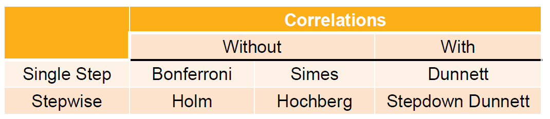
Single step methods
- The rejection or non-rejection of a single hypothesis does not depend on the decision on any other hypothesis.
- e.g. Bonferroni, Simes, Dunnett, etc.
-
Stepwise methods
- The rejection or non-rejection of a particular hypothesis may depend on the decision on other hypotheses.
- e.g. Holm, Hochberg, stepdown Dunnett, …
Methods
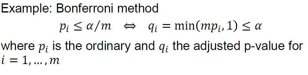
Bonferroni
- Use 𝛼/𝑚 for all inferences; for 𝑖=1,…,𝑚: $$\text{Reject } H_i \text{ if } p_i \le \alpha/m$$ or with adjusted p-values $q_i = \min(mp_i, 1)$, $$\text{Reject } H_i \text{ if } q_i \le \alpha$$
- This method follows the idea of Boole's inequality: $Pr(\cup A_i)\le \sum_i Pr(A_i)$, where $A_i = \{p_i\le \alpha/m\}$ denotes the event of rejecting $H_i$
- Properties
- Conservative if the number of hypotheses is large or the test statistics are strongly positively correlated
- Can be improved by using stepwise methods (e.g. Holm procedure) and accounting for correlations (e.g. Dunnett test)
- Rarely used in practice but is the basis for commonly used advanced procedures
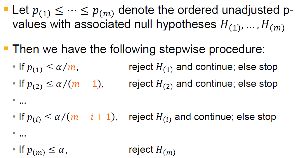
Holm
- Overview
- Using ordinary p-values
- Using ajusted p-values
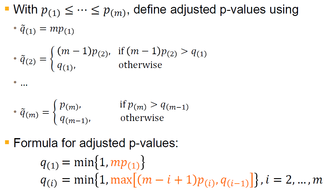
- Using ordinary p-values
- Properties
- A stepwise procedure and more powerful than Bonferroni method
- Sometimes called "stepdown Bonferroni" procedure
- Can be improved by accounting for correlations (e.g. stepdown Dunnett test)
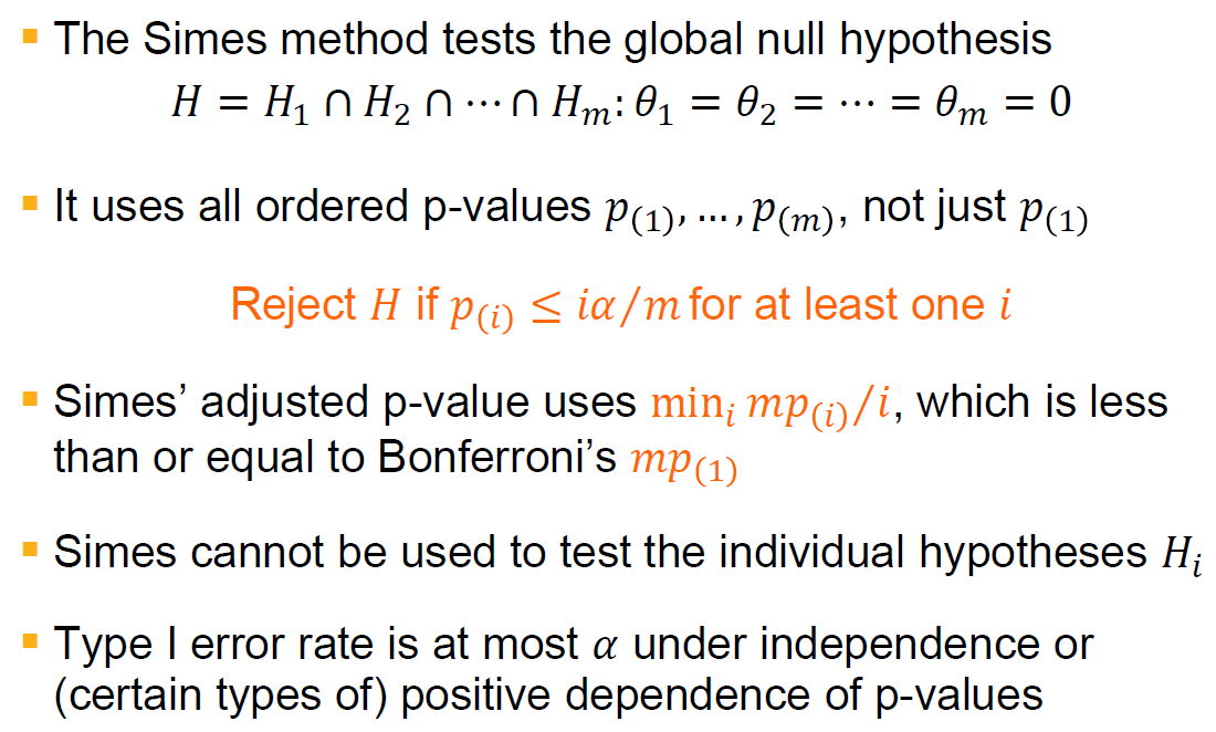
Simes
-
Overview
-
Comparison with Bonferroni
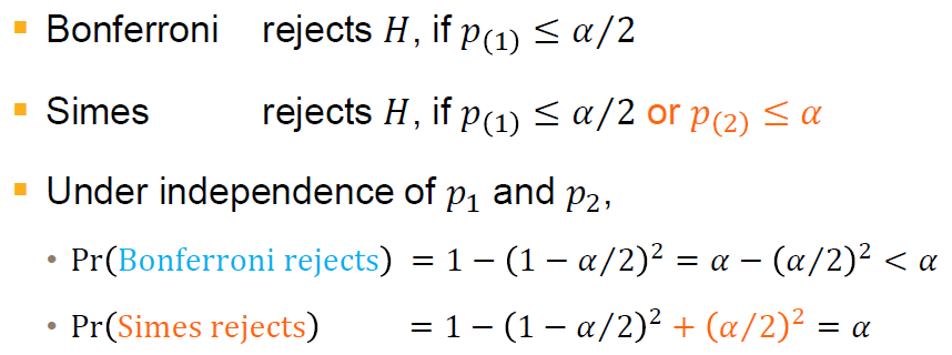
- Simes is more powerful than a global test based on Bonferroni
- Simes assumes non-negative correlations between p-values, Bonferroni doesn't
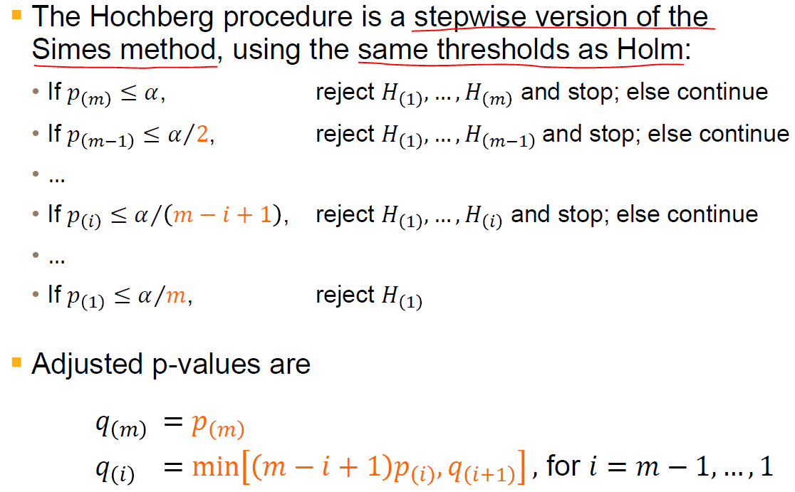
Hochberg (stepwise version of Simes method/stepup Simes)
- Overview
- Properties
- Stepup Simes
- More powerful than Holm procedure
- Both use same thresholds, but Hochberg starts with the largest p-value, whereas Holm starts with the smallest
- It makes same assumption as the Simes test, i.e. independence or positive dependence of p-values
- Can be improved, e.g. Hommel procedure based on the closed test procedure.
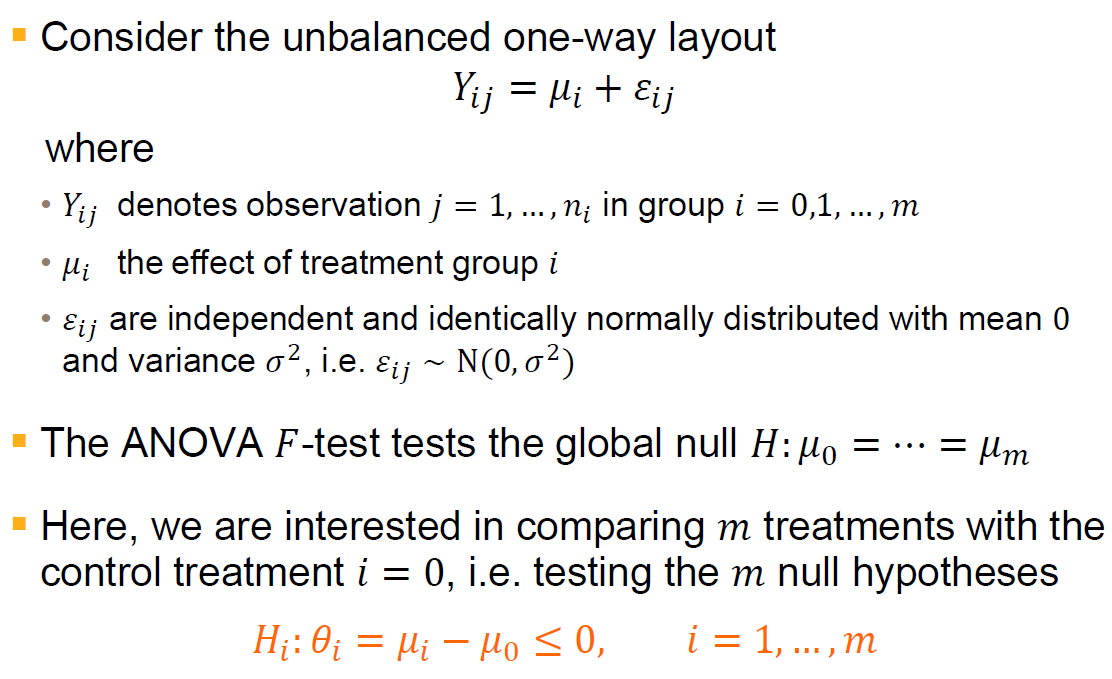
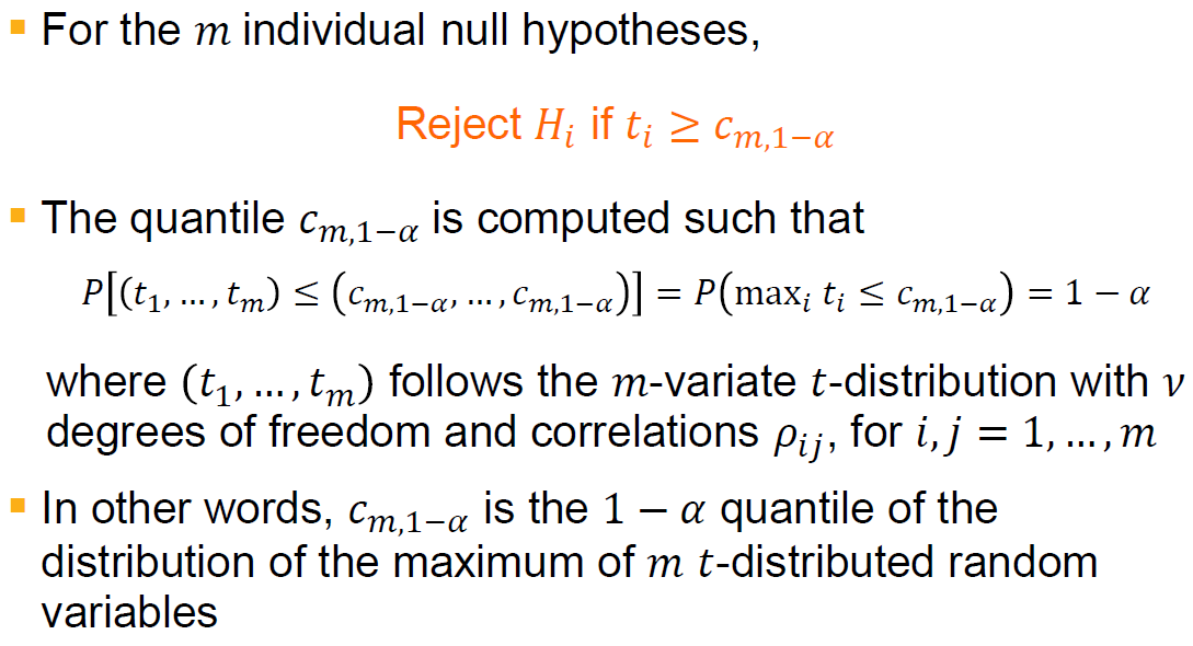
Dunnett
-
When comparing several treatments with a control
-
Other methods mentioned above can also be used but only Dunnett test exploits the correlation between the p-values
-
Overview
- linear model and hypotheses
- individual test statistics
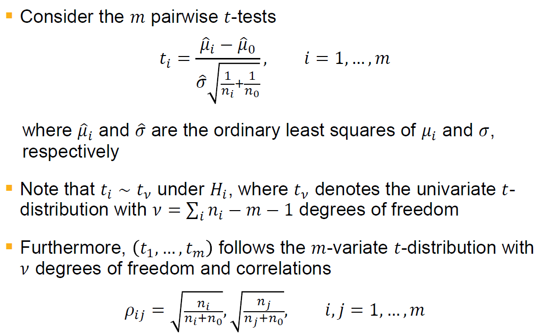
- rejection rule
- linear model and hypotheses
-
Properties
- Single step test, which is better than Bonferroni as it exploits the known correlations between test statistics
- Adjusted p-values can be calculated numerically based on the multivariate t-distribution
- The Dunnett test shown here can be extended to any linear and generalized linear model
- It can be improved by extending it to a stepwise procedure, similar to the Holm procedure
- Other well-known parametric tests follow the same principle. For example, the Tukey test compares all treatment groups against each other, also using a multivariate -distribution
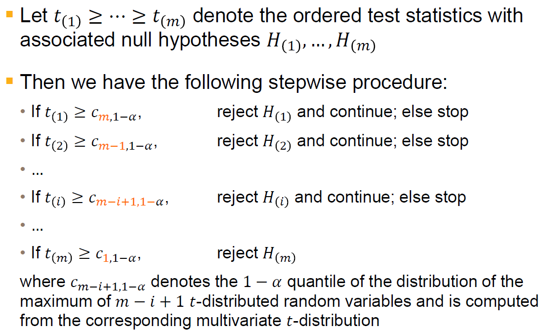
Stepwise Dunnett
-
Overview
-
Properties
- the quantiles change as hypotheses are rejected; e.g. if $H_{(1)}$ is rejected, then the quantile $c_{m-1, 1-\alpha}$ is computed from a (m-1)-variate t-distribution
- the stepwise Dunnett test is better than the single step Dunnett test
- it can be shown that $c_{m, 1-\alpha} \ge c_{m-1, 1-\alpha}\le \cdots \le c_{1, 1-\alpha}$, where $c_{1, 1-\alpha} = t_{v, 1-\alpha}$ is the quantile from the univariate t-distribution with $v$ degrees of freedom
- The Dunnett test uses $c_{m, 1-\alpha}$ for all comparisons
- the stepwise Dunnet test is better than the Holm procedure as it exploits the known correlations between test statistics
- The stepwise version shown here is sometimes called "stepdown Dunnett" test
- A "stepup Dunnett" test also exist, similar to Hochberg
Summary
- Stepwise methods are preferred over single step methods, which are less powerful and less used in practice
- Accounting for correlations leads to more powerful procedures, but correlations are not always known
- Simes-based methods are more powerful than Bonferroni-based methods, but control the FWER only under certain dependence structure
- In practice, we select the procedure that is not only powerful from a statistical perspective, but also appropriate from clinical perspective
Hierarchical test procedure
Background
- Previous multiple tests methods do not reflect the relative importance of the two endpoints, which is usually the case in RCT, where we have primary/secondary/exploratory endpoints with ordered importance
- Previous stepwise procedures use a data-driven order of hypotheses, whereas in the RCT setting we need a multiple test procedure that specifies the order of the hypothesis based on clinical importance
- Hierarchical test procedure: the hierarchy of hypotheses is specified before data is observed
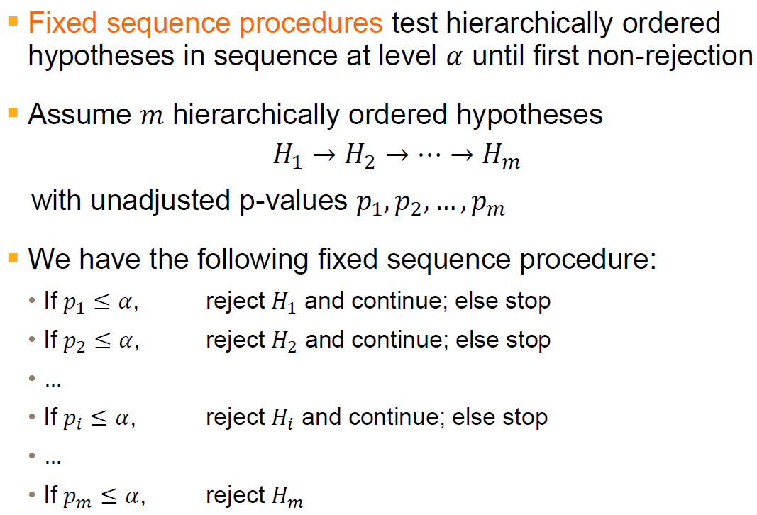
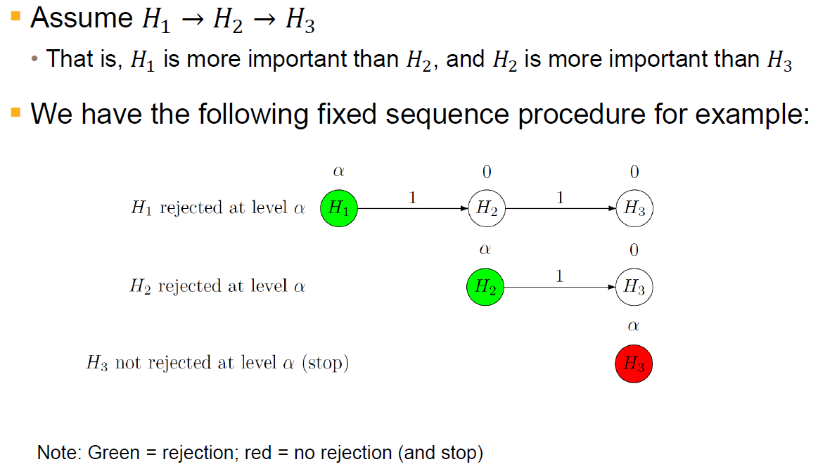
Fixed sequence procedure
-
Overview
-
Properties
- Adjusted p-values are given by $q_i = \max\{p_1, \cdots, p_i\}, i = 1, \cdots, m$
- Advantages
- Simple
- Optimal when hypotheses early in the sequence are associated with large effects and performs poorly otherwise
- Disadvantages
- Once a hypothesis is not rejected, no further testing is permitted
- Great care is advised when specifying the sequence of hypotheses
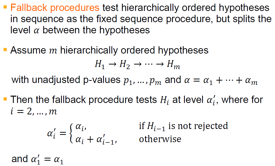
Fallback procedure
-
Overview
-
Properties
- The fixed sequence procedure is obtained as a special case from the fallback procedure by setting $\alpha_1=\alpha$ and $\alpha_i=0$ for $i>1$
- In contrast to the fixed sequence procedure, fallback procedure tests all hypotheses in the pre-specified sequence even if the intitial hypotheses are not rejected
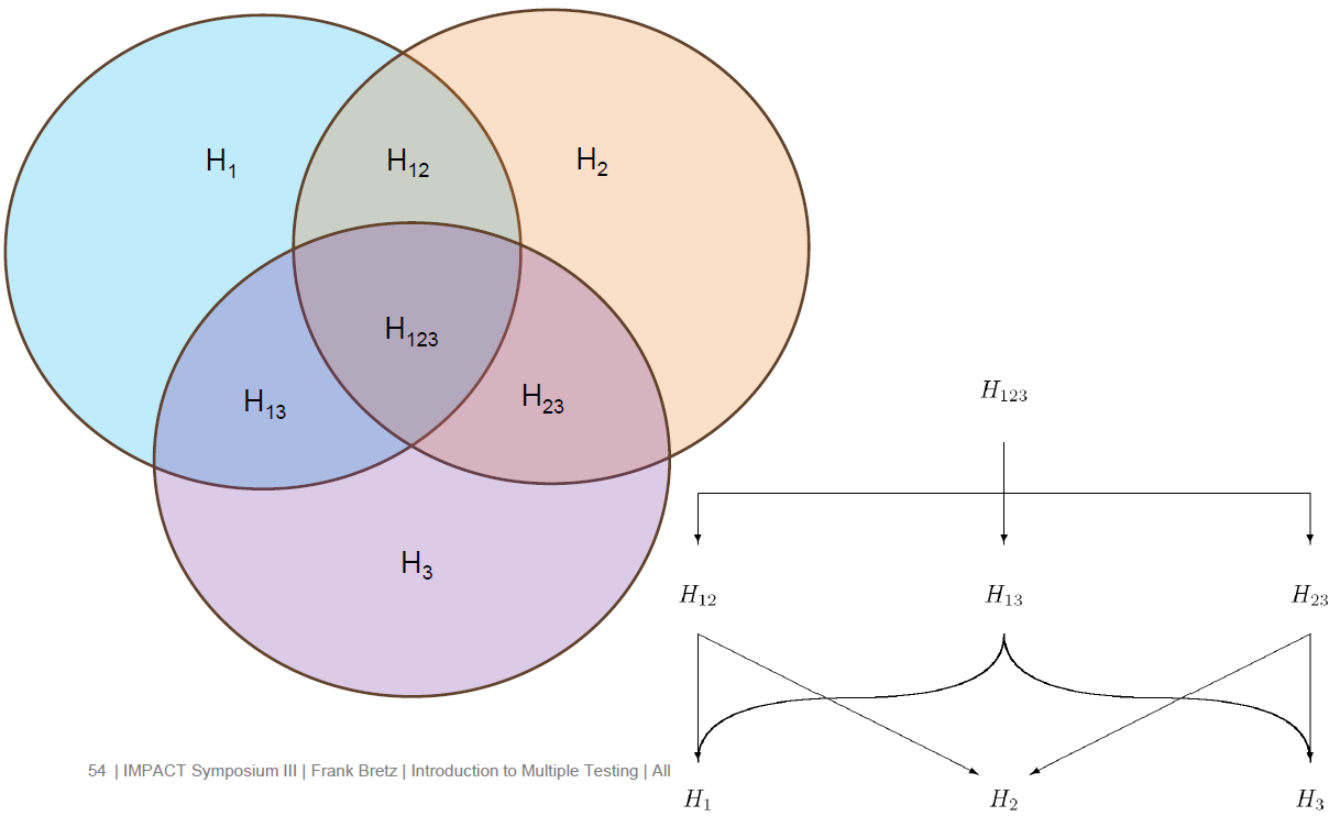
Closed test procedure (CTP)
- Overview/formal definition
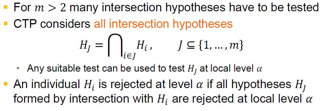
- Test the iteraction hypotheses using Bonferroni, Simes, Dunnett, etc. at level $\alpha$
- Test each individual hypothesis at level $\alpha$
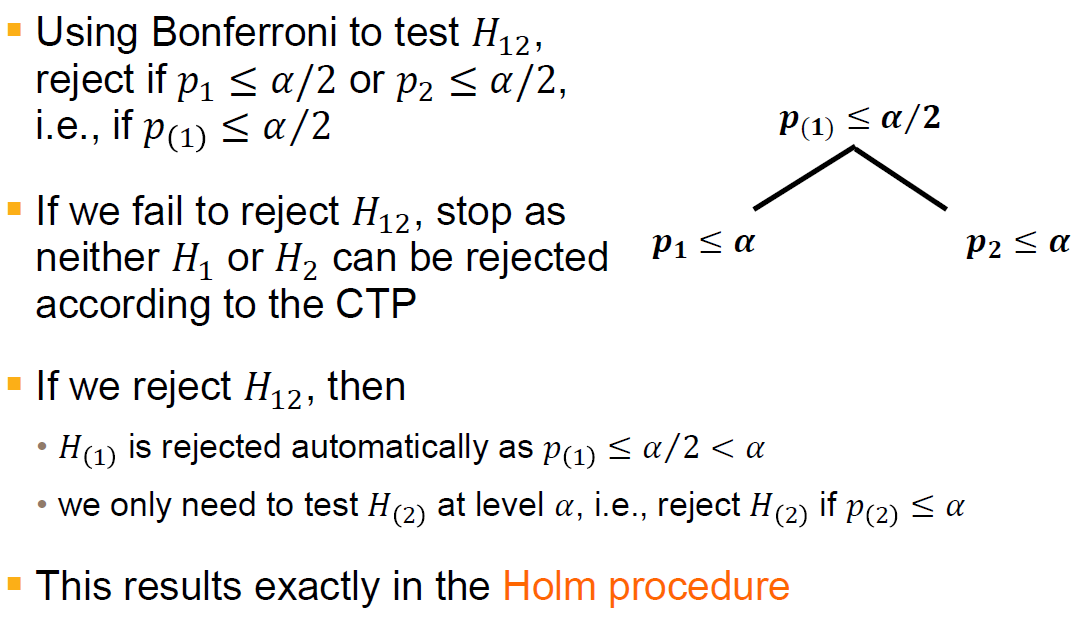
CTP using Bonferroni ( == Holm procedure)
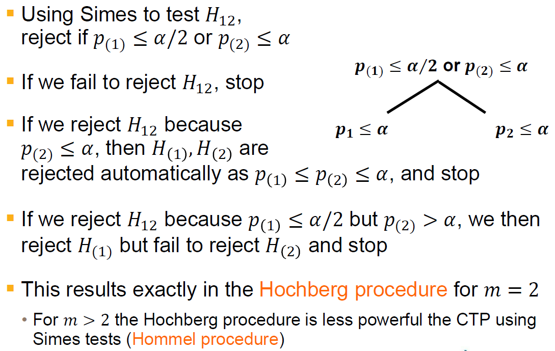
CTP usign Simes
- When m=2, it's equivalent to Hochberg procedure
- When m>2, it's less powerful
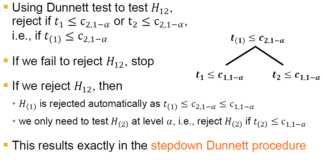
CTP using Dunnett
- This is equivalent to stepdown Dunnett procedure
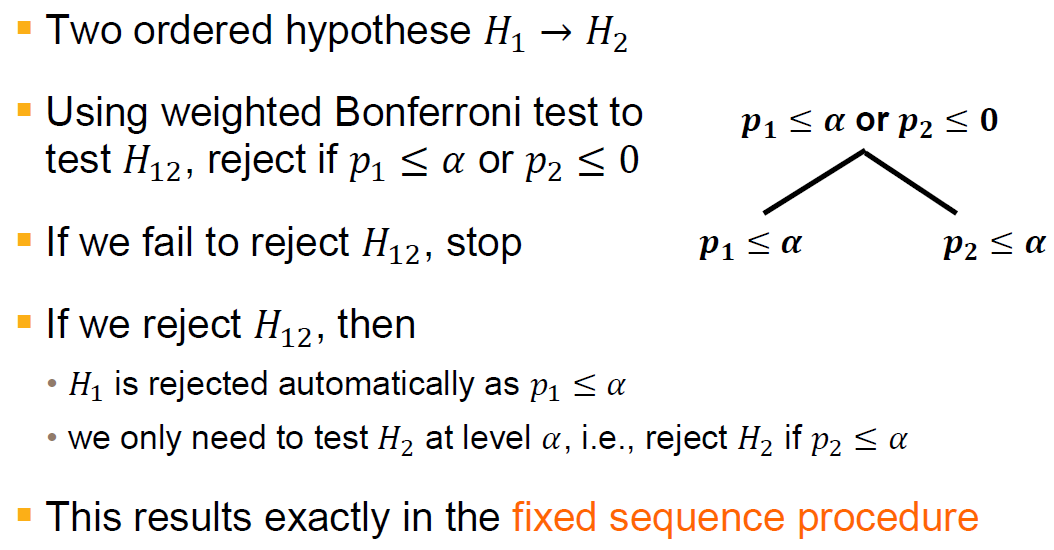
CTP using weighted Bonferroni
-
The first is equivalent to the the fixed sequence procedure
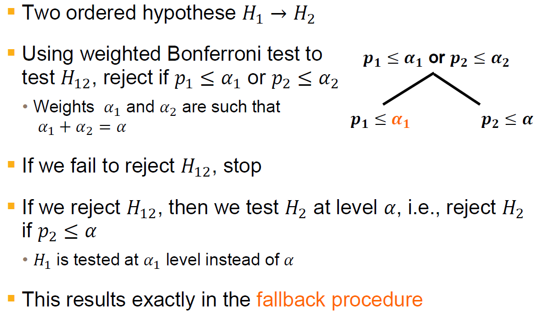
-
The second version is equivalent to the fallback procedure
What if more than two hypotheses?
- Do CTP for pairwise combinations
Summary
Summary and Conclusions
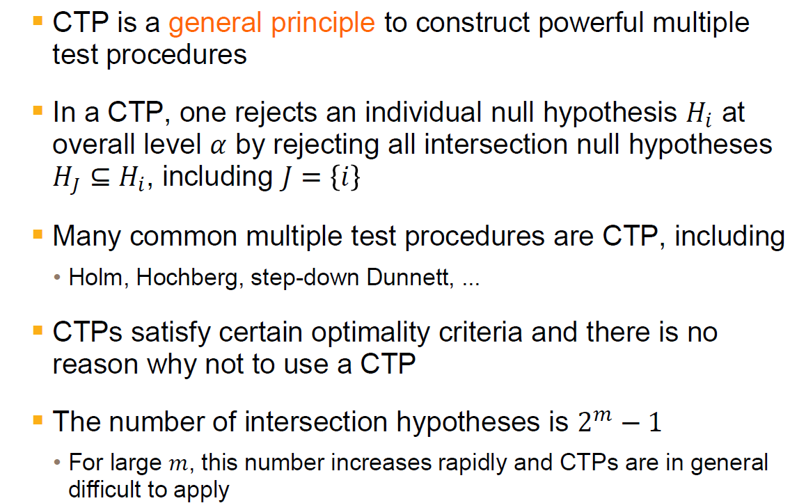
- Closed test procedure is a general principle to construct powerful multiple test procedures; many common procedures are CTPs
- For structured hypotheses, one can apply the graphical approach, which is based on CTPs
- It is critical to choose the suitable method for a particular problem
- There are different types of multiplicity problems that need other methods than those described here, such as:
- Safety data analyses
- Large-scale testing in genetics, proteomics etc.
- Post-hoc analyses / data snooping
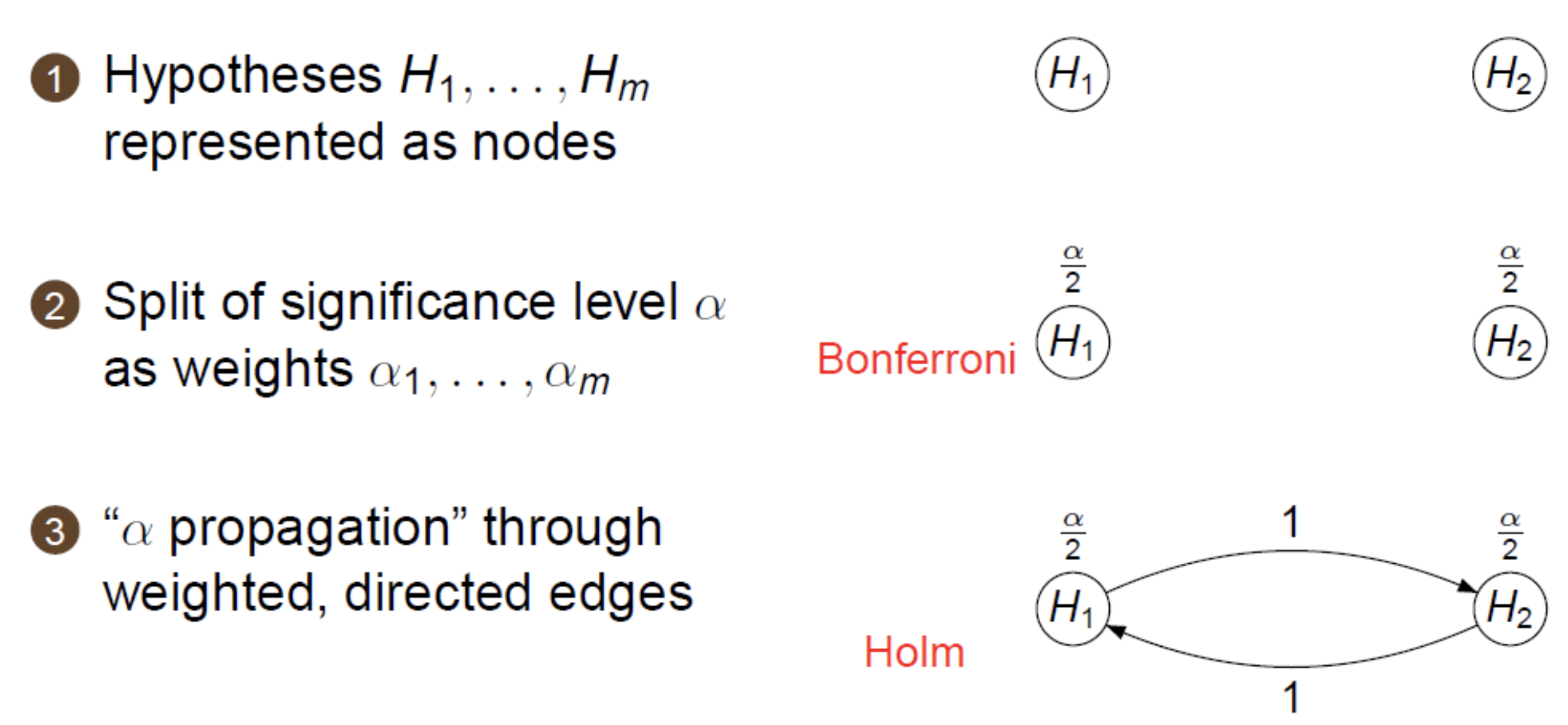
Graphical approach[1][2]
- Initial allocation of the significance level to $m$ hypothesis: $\alpha_1 + \cdots + \alpha_m = \alpha$
- $\alpha$-propagation: if a hypothesis $H_i$ is rejected at level $\alpha_i$, propagate its level $\alpha_i$ to the remaining, not yet rejected hypotheses (according to aprefixed rule) and continue testing with the updated $\alpha$ levels
Conventions
Weighted Holm procedure: i.e. $\alpha$ is no longer evenly splited among hypotheses
Common multiple test procedues
- Fixed sequence procedure
- Fallback procedure
Formal description
-
Initial levels $\alpha = (\alpha_1, \cdots, \alpha_m)$ with $\sum_{i=1}^m\alpha_i = \alpha \in (0, 1)$
-
$m \times m$ Transition matrix $\bf{G}=(g_{ij})$, Where $g_{ij}$ is the fraction of the level of $H_i$ that is propagated to $H_j$ with $0\le g_{ij} \le 1, g_{ii} = 0$ and $\sum_{j=1}^mg_{ij}\le1, \forall i=1, \cdots, m$
($G, a$) determine a graph with an associated multiple test
-
Update algorithm
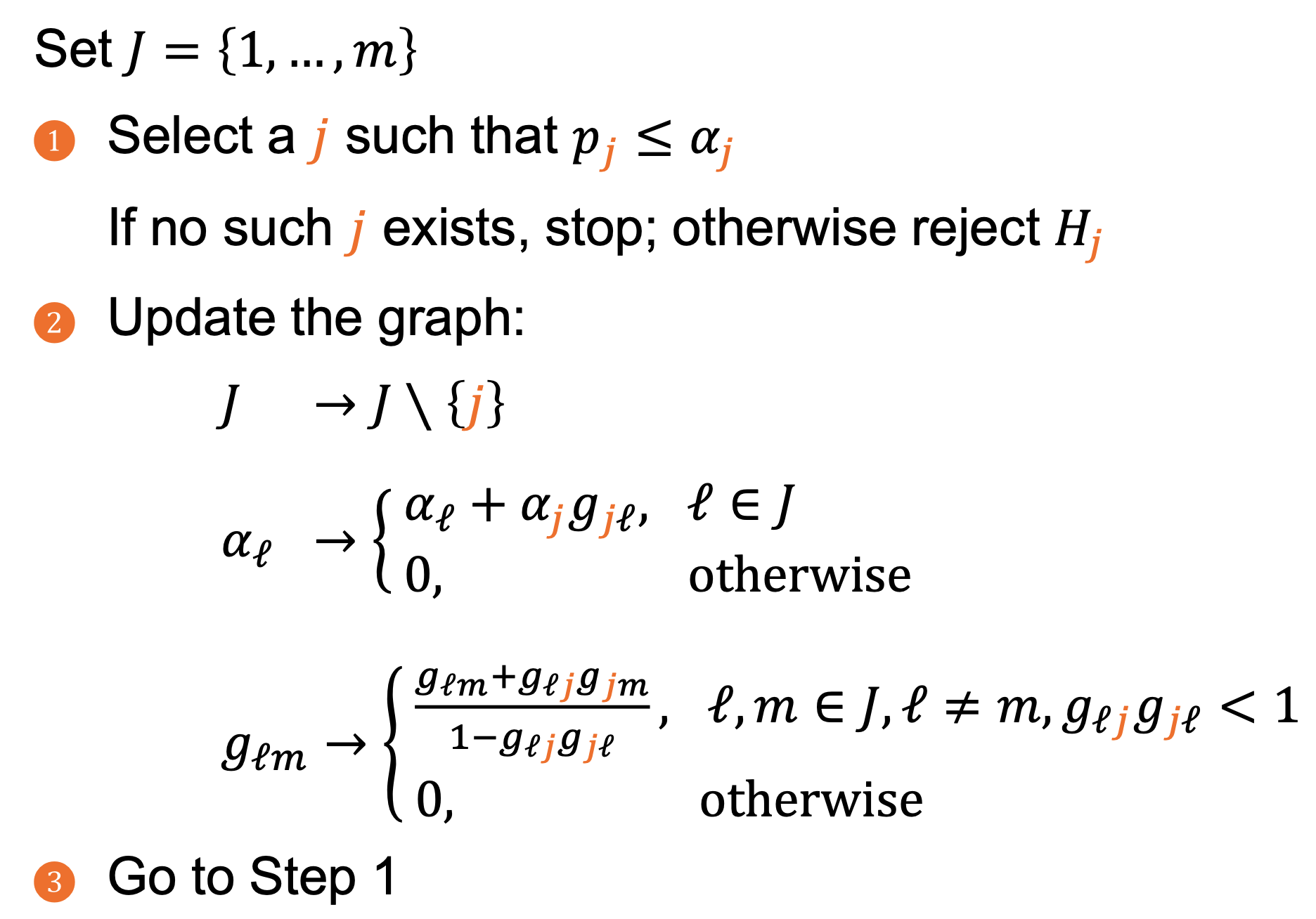
-
The initial levels $\alpha$, the transition matrix 𝑮, and the algorithm define a unique sequentially rejective test procedure that controls the FWER at level $\alpha$
-
Any multiple test procedure derived and visualized by a graph ($G, \alpha$) is based on the closed test principle
-
The graph ($G, \alpha$) and the algorithm define weighted Bonferroni tests for each intersection hypothsis in a CTP
-
The algorithm defines a shortcut for the resulting CTP, which does not depend on the rejection sequence
-
Tools:
R{gMPA} package
Summary
- Tailor advanced multiple test procedures to structured families of hypotheses
- Visualize complex decision strategies in an efficient and easily communicable way
- Ensure strong FWER control
- It covers many common multiple test procedures as specifal cases: Holm, fixed sequence, fallback, gatekeeping, etc.
References
Bretz, Frank and Maurer, Willi and Brannath, Werner and Posch, Martin (2009). A graphical approach to sequentially rejective multiple test procedures. ↩︎
Bretz, Frank and Posch, Martin and Glimm, Ekkehard and Klinglmueller, Florian and Maurer, Willi and Rohmeyer, Kornelius (2011). Graphical approaches for multiple comparison procedures using weighted Bonferroni, Simes, or parametric tests. ↩︎